Differential geometry of ML
Machine learning has achieved remarkable advancements largely due to the success of gradient descent algorithms. To gain deeper mathematical insight into these algorithms, it is essential to adopt an accurate geometric perspective. In this article, we introduce the fundamental notion of a manifold as a mathematical abstraction of continuous spaces. By providing a clear geometric interpretation of gradient descent within this manifold framework, we aim to help readers develop a precise understanding of gradient descent algorithms.
To explain manifolds in the simplest way, a manifold is the most concise mathematical model for understanding “continuous spaces.” But what does “continuous” mean?
Let’s consider this through an example. Suppose there is a point in space, and I have degrees of freedom to move this point, so that I can move the point continuously. Then, every point in the neighborhood of that point can be uniquely obtained by appropriately adjusting the weights of those degrees of freedom (they can be parameterized). To express this concisely in mathematical terms:
“The space around a point in the space is somehow looks like .”
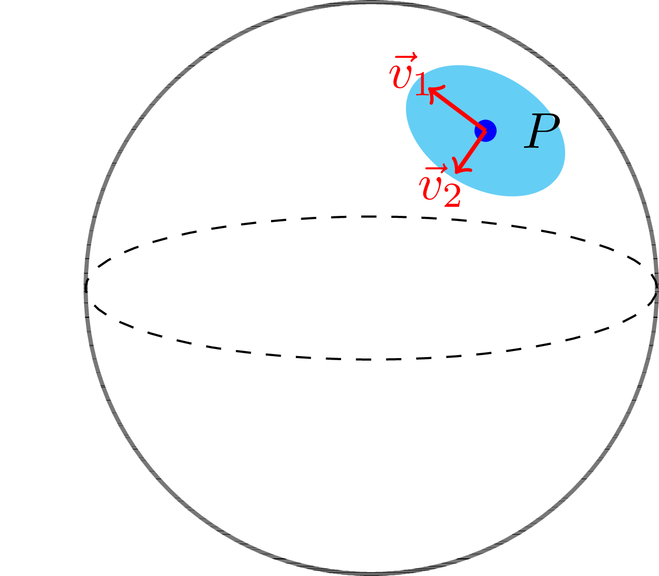
Figure 1: 2D sphere with a point . We can locally perturb with two independent directions , .
With this philosophy, we can define a manifold as follows:
“When the space around every point in a space looks like Euclidean space, we call this space a manifold.”
In this case, if the space around every point p can be continuously obtained by degrees of freedom, we define the dimension of this manifold to be .
Here are some concrete examples of manifolds.
Example 1 (The sphere ) The sphere is a manifold, because we can “smoothly” flatten it to a plane, locally.
Example 2 (regular value) From the previous example, we can see that the sphere is a manifold. Actually, the sphere can be defined by the equation . Equivalently, if we define by , then the sphere is .
In general, for any smooth function , a point is called a regular point of if the gradient . For , it is called a regular value of if all points in are regular points. Then, the regular level set theorem says that for any regular value , the level set is a manifold [6].
Example 3 (Torus) For , consider the torus contained in parametrized by
for . This is a smooth manifold, because intuitively, we can cover the torus with smooth charts. On the other hand, it can also be proved by taking the function defined by and checking that the level set is a smooth manifold.
Goal of this post
If we have a space called a manifold, we can consider various mathematical objects on that space. The mathematical objects of a manifold are concepts that extend from objects in Euclidean space, which is the local model (by ‘local’ we mean information about how the space around every point in the space looks). The basic geometric objects in the euclidean space are …
- The euclidean space .
- The vector field on .
- The covector field on .
- Euclidean metric on .
Our goal is to understand these objects, and generalize these things by replacing the space with an arbitrary smooth manifold .
Tangent vectors, Tangent space
“For Euclidean space , the commonly understood concepts of tangent vectors and tangent spaces are as follows:”
- A tangent vector at a single point is a vector attached at that point.
- A tangent space at each point is a duplicate of , attached to each point. (This is the space where tangent vector is living.)
- A vector field is a collection of tangent vectors, attached to each point, or equivalently, a map that assigns a tangent vector to each point.
We must convert these notions to the general manifold . To do so, we need to understand the notion of tangent vector in a new way.
Philosophy 1
A tangent vector at = An infinitesimal movement at = Differential operator at
Correspondence 1 (tangent vector ↔ infinitesimal movement) If a vector is attached to a point, we can move the point for a very short moment in the direction of that vector. Conversely, if a point moves slightly for a very short moment, the derivative in the direction of that movement becomes a vector. This is the correspondence between tangent vectors and infinitesimal movements.
Correspondence 2 (infinitesimal movement ↔ differential operator) Local movement can be understood as a differential operator. A differential operator means that when there is a function , we differentiate appropriately. In other words, if we want to understand local movement as a differential operator, we need to make the local movement act on any function . If we move locally from point to , we can observe the amount by which the function value of changes due to this movement, and this becomes a first-order differential operator acting on . Conversely, the fact that any differential operator actually comes from local movement is beyond the scope of this discussion, so we will omit the proof.
In this perspective, we can generalize the notion of tangent vector to an arbitrary smooth manifold.
- A tangent vector at a single point is a differential operator at that point.
- A tangent space at each point is a vector space of differential operators at that point.
- A vector field is a collection of differential operators, attached to each point, or equivalently, a map that assigns a differential operator to each point.
Example 4 Consider the Euclidean space . Suppose we have a vector field . We now understand this as a differential operator , which acts on a smooth function as
Now, we introduce a notion that might be unfamiliar to some readers, which is the notion of a cotangent vector. A cotangent vector is basically a linear measurement of tangent vectors. Mathematically, it can be written as:
Definition (Cotangent vector) Let be a manifold. Let be a point, and let be the tangent space at . A cotangent vector at is a linear map . We denote the space of cotangent vectors at by . (By definition, it is a dual space of .)
It might seem very unnatural to define a cotangent space at first glance, but it turns out that it is a very natural notion, since it is equipped with a canonical object called the differential of a smooth function.
Example 5 (Differential of a smooth function) Let be a manifold. Let be a point, and let be a smooth function. The differential of at is a linear map , defined by Now, we can understand as follows. is an object that contains the information of the first derivative of at , and if we put a direction into , it returns the derivative of in that direction. That is, any function on a manifold actually has the ability to linearly measure tangent vectors, and therefore can function as a cotangent vector.
Similar to the case of vector space, we can define the notion of cotangent space, vector and field to an arbitrary smooth manifold.
- A cotangent space at each point is the dual vector space of tangent space at that point.
- A cotangent vector at a single point is an element of cotangent space at that point.
- A cotangent vector field is a collection of cotangent vectors, attached to each point, or equivalently, a map that assigns a cotangent vector to each point.
The remaining object is a metric; we need to understand how can we define a metric on a manifold. To do so, we first need to understand what is a canonical bundle over a smooth manifold.
What is a tensor bundle?
In the previous section, we defined the notion of tangent space and cotangent space. Using these objects, we can define a tangent bundle and a cotangent bundle over a smooth manifold.
Definition (Tangent bundle, cotangent bundle) Let be a smooth manifold. The tangent bundle of is the set of all tangent spaces at each point, i.e. The cotangent bundle of is the set of all cotangent spaces at each point, i.e.
The easiest way to understand bundles is to think of a bundle as an object that is actually formed by collecting and gluing together Euclidean spaces. For example, in the case of a 2-dimensional surface, the manifold itself has 2 degrees of freedom, and since there is a 2-dimensional tangent space at each point, when we attach additional 2-dimensional spaces with two more degrees of freedom, we get a 4-dimensional space, and that becomes the tangent bundle of that surface.
This object called the tangent bundle has one more nice property in addition to the characteristic that it becomes a manifold itself. Before explaining this, let us first define what a fiber is.
Definition (fiber) For two manifolds , , consider a continuous function . For a point in , we define as the fiber of .
Now let us examine one more nice property of the tangent(cotangent) bundle.
Property Let be a manifold, and let () be the tangent bundle (cotangent bundle, respectively). Then has an -dimensional vector space structure on each fiber.
We call the manifold with the map satisfying the property that each fiber has a vector space structure a vector bundle over . From this perspective, and are vector bundles over . The following are simple properties of vector bundles.
Proposition Let be a vector bundle over . Then, is a smooth manifold.
- We can define a dual bundle of .
- We can define a tensor product bundle of and .
For those who are not familiar with dual spaces and tensor products, in the next section we will briefly review these concepts.
Dual space, Tensor product
For a vector space , consider the collection of all linear functions from that vector space to the real numbers . If we fix , then for a real number , is also a linear function from to the real numbers, and therefore has a natural vector space structure. We define this space as the dual space of .
Example 6 Consider the vector space . What does the dual space of this space look like? First, the easiest basis to think of in this space is . Now let us define as follows:
That is, becomes the projection onto the i-th coordinate. We can easily see that linear combinations of the ‘s constitute , and therefore
When there are two vector spaces and , let the basis of be , … , and the basis of be , … . In this case, we want to define a vector space that combines the spaces and to have pairs as a basis. In more mathematical notation, we express the basis as , and write the space created by combining these bases as .
Using dual spaces and tensor products, we can understand matrices mathematically. If and , then we understand linear functions from to as matrices. Then what does the element in the -th row and -th column of this matrix mean? Consider a matrix that has 1 written only in the -th row and -th column position, and 0 in all other positions. If we examine the mechanism by which this matrix acts when applied to an element of , it first performs a projection onto the -th coordinate of , and then outputs that value to the -th coordinate of . Expressing this from the tensor product perspective, we can think of . Since these matrices form a basis for the space of all linear functions from to , we have
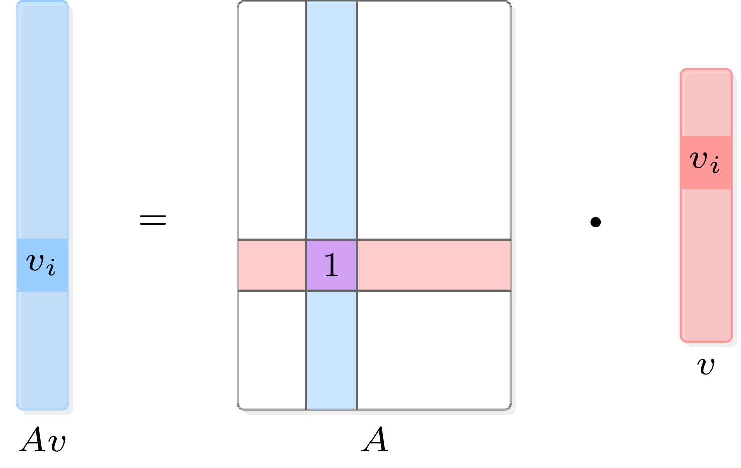
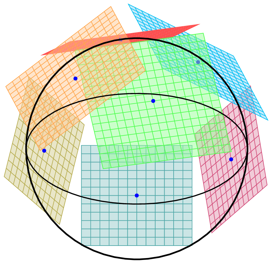
Figure 4: Visualization of a canonical basis of matrix space. This visually shows the equation .
Return to Bundle
Returning to the discussion, we can now understand the dual of vector bundles and tensor products between vector bundles. We can perform operations on the vector spaces corresponding to the fibers at each point of the manifold, then collect and glue together all the vector spaces that have undergone these operations to create new vector bundles. What we obtain in this way are the and defined above.
Recall that and are objects that are defined as soon as we define . Then from the perspective of the above proposition, is an object that is immediately defined over . We call such a canonical vector bundle a tensor bundle.
Now, we can understand tangent fields and cotangent fields as objects defined from sections of bundles.
Definition (section of a vector bundle) Let be a vector bundle. A section of is a map such that for all .
In other words, a section of a vector bundle is a map that assigns a vector in the fiber to each point of the manifold. Therefore, tangent field and cotangent field can be re-defined as follows.
Definition (tangent field, cotangent field) Let be a manifold. A tangent field on is a section of , and a cotangent field on is a section of .
Canonical operations on differential geometry
Given a map , how the objects like tangent vector and cotangent vector move canonically by the map ?
Philosophy A map between two manifolds “push” tangent vectors and “pull” cotangent vectors.
To explain, we check how push and pull such vectors, explicitly. We start with the pushforward of a tangent vector.
Definition Let be a smooth map. For each , the pushforward of a tangent vector is a tangent vector , which is a differential operator acts on smooth function as
Example 7 Suppose we have a smooth map . For a tangent vector , we calculate the pushforward . Take a function , and we have Therefore, .
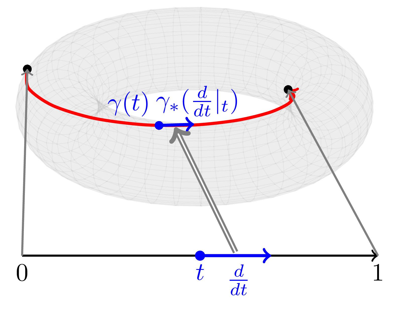
Example 8 When we have a manifold and a point on it, intuitively, a differential operator at measures the rate of change of a function along a local path passing through . Let’s write this in a mathematically rigorous way. A path through is mathematically expressed as a parametrized path with . Now, the differential operator we intuitively thought about above is actually . Mathematically verifying this, for a smooth function , we have
That is, is an operator that gives the derivative of along the path .
Since a smooth map pushes vectors, from the perspective of tangent spaces, we can see that it defines a linear map that pushes between tangent spaces.
Definition Let be a smooth map. For each , the differential of at is a linear map which maps a tangent vector to a tangent vector defined by
Example 9 Let be a smooth map. From the previous example, we have Therefore, is a linear map which maps Here, we see that is a matrix that represents the map . This matrix is called the Jacobian matrix of at .
Now, we see how the smooth map acts on cotangent vectors. Intuitively, a cotangent space is a dual space of a tangent space, so the natural direction of the action should be reversed. Therefore, we may infer that the smooth map will pull cotangent vectors.
Definition Let be a smooth map. For each , the pullback of a cotangent vector is a cotangent vector , which is a linear map defined by
Example 10 In the previous example, we defined the differential of a smooth real-valued function on a manifold. At that time, we saw that this object is a cotangent vector field. In fact, this object can be understood as a pullback. First, let’s define a canonical cotangent vector field on the real line that satisfies the following: Now, let’s prove that the pullback of this dt using f is df. Fix p in M. Take a tangent vector at p. Then, We claim that . To see this, we take any smooth function , by chain rule, Therefore, going back to the above equation,
So far, we have examined how acts on tangent vectors and cotangent vectors. Now, let’s describe this at the level of tangent bundles and cotangent bundles. Before that, let’s first define a morphism between vector bundles.
Definition (morphism of vector bundles) Let and be vector bundles. A smooth map between vector bundles together with a map is called a morphism of vector bundles if
- maps each fiber of to a fiber of . Precisely, let be a point, and let be the fiber of at . Then, .
- is a linear map.
Example 11 Let be a smooth map. Then, the pushforward induces a morphism of vector bundles. This map vector bundle morphism is defined as follows:
Unfortunately, the pullback does not induce a morphism of vector bundles, since there is no map from to . However, we still can construct a canonical object.
Definition (Global section of a vector bundle) Let be a vector bundle over . The global section of is a map such that for all . The collection of all smooth global sections of is denoted by .
Example 12 Let be a smooth manifold. The collection of all smooth vector fields on is .
Example 13 Let be a smooth manifold. Let be a smooth function. Then, the differential is an element of .
Definition (Pullback of a global section) Let be a smooth map. Take . Then, the pullback of is a global section of , which is defined by Therefore, induces a map .
Therefore, given a smooth map , we have canonical maps
- .
It can be shown that these can be extended to tensor bundles: For positive integer , we have canonical maps
- .
What is a metric?
In the previous section, we studied various geometric objects on a smooth manifold, including bundles and global sections. In this section, we will study a metric on a smooth manifold, and understand it as a global section of a tensor bundle. To do so, we first see the easiest example of a metric, which is the Euclidean distance arising from an inner product on a vector space.
Definition (Inner product) Let be a vector space. An inner product on is a map that satisfies the following properties:
- Bilinearity: for all and .
- Symmetry: for all .
- Positive-definiteness: for all , and if and only if .
Then, we can equip a vector space with a norm by and this norm induces a metric on .
What is important here are two things:
- An inner product is symmetric, bilinear, and positive-definite.
- An inner product takes two vectors and returns a real number.
When a vector space is given, since an inner product is an operator that takes two vectors and outputs a single real value, it can be understood as an element of . Then, when we think from the perspective of manifolds and tangent bundles on them, we can intuitively understand that a metric on a manifold is a 2-tensor field, i.e. an object that takes two tangent vectors and returns a real number at each point, or 2-cotangent vectors at each point of the manifold. More rigorously, this can be written as follows.
Definition (Metric) [7] Let be a smooth manifold. A metric on is a global section of which is bilinear, symmetric, and positive-definite.
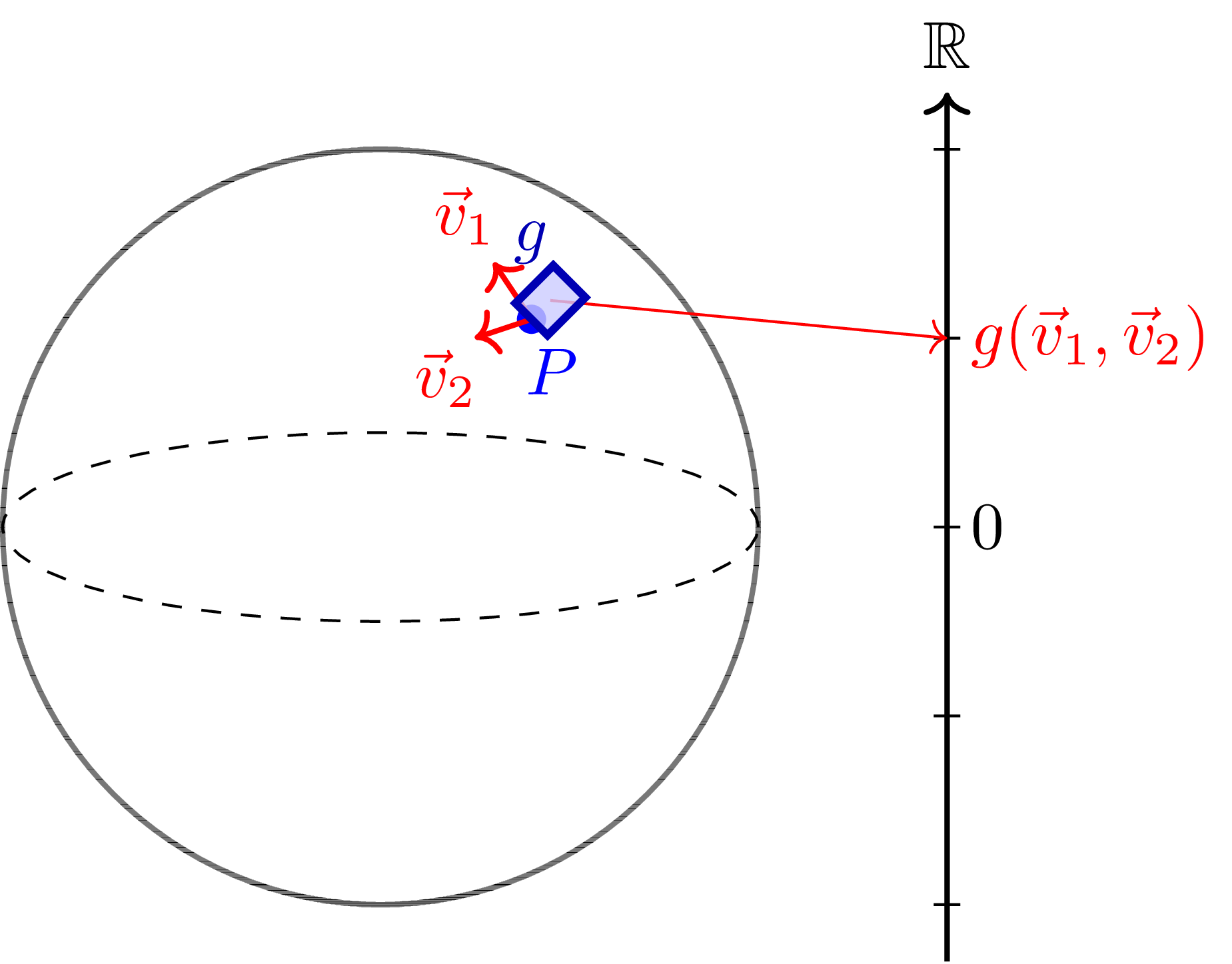
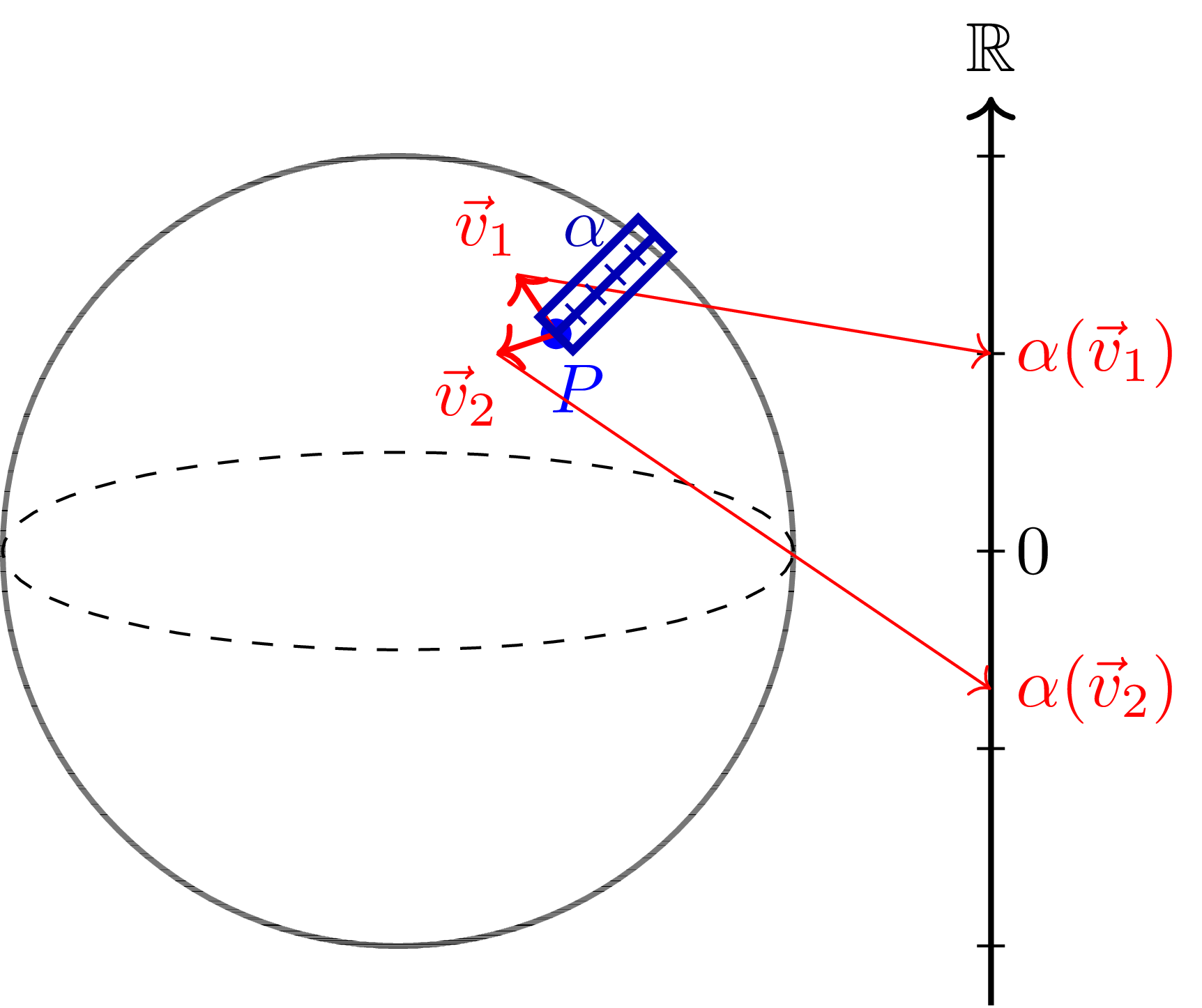
Figure 6: A metric on a sphere. At a point , takes two tangent vectors and gives one real value.
Example 14 The standard metric on is given by where is the differential of the -th coordinate function . Fix . Suppose we have a tangent vector . Then, we have Since a tangent vector represents an infinitesimal direction of change, this value can be understood as the square of the infinitesimal change in the tangent direction.
From this definition, we can calculate the length of a curve explicitly.
Example 15 (Length of a curve) Let be a smooth manifold. Let be a curve. The length of is given by Here, is a tangent vector at the point , tangent to the curve , defined by
One common misconception is thinking that when there is a manifold and a function on it, there naturally exists an object called the gradient. This is incorrect; a gradient only exists when there is a metric on the manifold. In fact, as we saw in the previous section, when there is a function on a manifold, the naturally existing object is the differential of the function, which belongs to . That is, since a gradient is a vector field, we can only consider a gradient when there exists a means to transfer objects in to .
When there is a vector space with an inner product , we can define an isomorphism between the vector space and its dual space as follows: Through this, we can view elements of the dual space of vector space as elements of vector space .
Using this, when there is a metric , we can define a bundle isomorphism as follows:
Definition (Gradient) Let be a smooth manifold. Let be a smooth function. The gradient of is a vector field on defined by
Example 16 Consider the Euclidean space , equipped with the standard metric . Consider a smooth function . Then, the differential of is given by Therefore, the gradient of is given by
We will understand the gradient from another perspective and end this section.
Definition Let be a smooth manifold. Let be a metric on . The metric induces a tensor by
Example 17 Consider the Euclidean space , equipped with the standard metric . Then, the metric induces a tensor , which is given by
Definition (gradient using ) Let be a smooth manifold. Let be a metric on . The gradient of a smooth function using is given by Here, is a 2-tensor, so applying it to a 1-covector will give a 1-tensor, which is a tangent vector.
Example 18 Consider the Euclidean space , equipped with the standard metric . Then, the gradient of a smooth function using is given by This is identical to the gradient of in the previous example.
Differential geometric setting for DNN
This section is to define mathematical objects that appear in deep learning, and understand them geometrically.
- Let be a input space.
- Let be a output space.
- Let be a space of functions from to .
- Let be a manifold of parameters. We use to denote a point in .
- Let be a model, which is a map .
- Let be a loss function.
Since DNNs use a gradient descent method to optimize the parameters, we understand that the parameter space must be equipped with a metric.
Remark The spaces , , and are usually chosen as Euclidean spaces. Therefore, is also a vector space (vector space of functions) Since a tangent space of a vector space can be identified with itself, all of their tangent spaces are canonically identified with themselves.
Remark Different metrics assigned to induce different optimization algorithms. For example, when is equipped with a Euclidean metric, the optimization algorithm is standard gradient descent. However, by assigning a spectral norm (of matrix space), we obtain some different optimization algorithms like muon or shampoo [3],[4],[5].
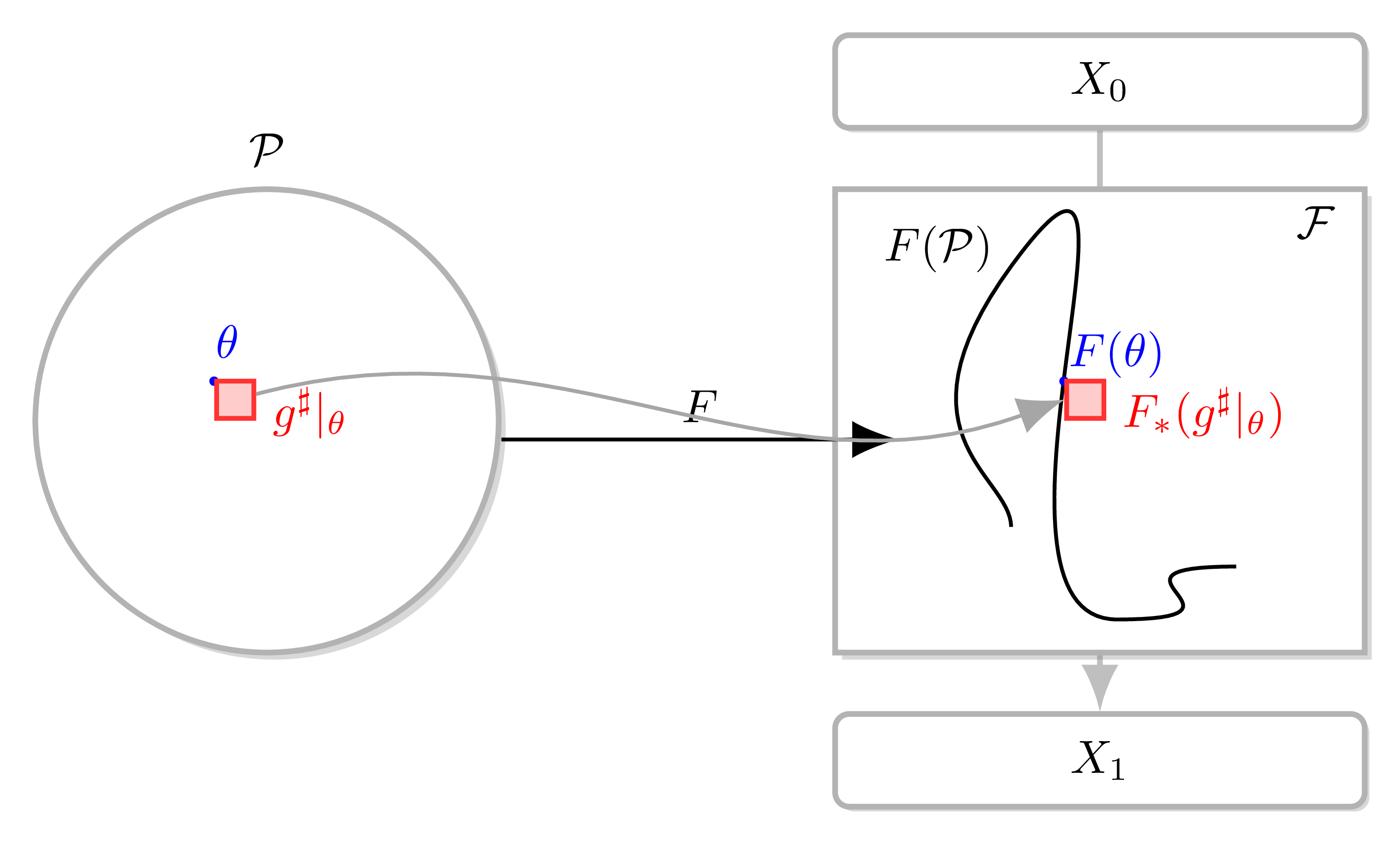
Figure 7: A model pushes the 2-tensor to the NTK living over the function space .
Neural Tangent Kernel
The strength of this framework is that we can understand NTK directly. NTK is fundamentally an approach that understands parameter changes not as parameter changes but as function changes [1],[2].
Definition (Neural Tangent Kernel) Let be a model. Let be a metric on . The NTK at is .
Recall the previous definition. We can understand the gradient of using 2-tensor . In the DNN setting, there is a gradient flow on , and this gradient is with respect to the composition of . That is, we can understand this gradient flow by taking the differential of and compute with . If we want to view this flow not on but on , we pushforward the whole situation to , obtaining a vector flow by computing the differential of with the pushforward of . In other words, NTK is what allows us to view the gradient flow in the sense of function space.
We also verify this definition is equivalent to the one in the literature by explicit calculation.
Example 19 By equipping with a Euclidean metric, we have From [2], we have Therefore, they are identical.
References
[1] Arora, Sanjeev et al. On Exact Computation with an Infinitely Wide Neural Net. NeurIPS 2019.
[2] Arthur Jacot, Franck Gabriel, Clément Hongler, Neural Tangent Kernel: Convergence and Generalization in Neural Networks, arXiv:1806.07572
[3] Gupta, Vineet, et al. “Shampoo: Preconditioned stochastic tensor optimization” (2018)
[4] Jeremy Bernstein and Laker Newhouse. “Old optimizer, new norm: An anthology.” arXiv preprint arXiv:2409.20325 (2024).
[5] Jordan Keller, Muon: A Matrix Norm Optimizer for Deep Learning, https://kellerjordan.github.io/posts/muon/
[6] Lee, John M. Introduction to Smooth Manifolds, (2002)
[7] Lee, John M. Introduction to Riemannian Manifolds, (2018)